Problem 12 : Residue Theorem

Complex numbers have enormous significance in several problems in engineering (e.g. 2-D irrotational and incompressible flow) and mathematics (e.g. Integrals, Probability). The familiar representation \(u + iv\) brings several things to our mind. It can be thought of merely as a complex number, represented as a point on the complex plane or even considered to be a vector with x-component equals \(u\) and y-component equals \(v\).

Integral of a complex function ? What’s that?

Many of us who’ve gone through university-level preliminary mathematics courses may have compress across contour integrals like the one given below :

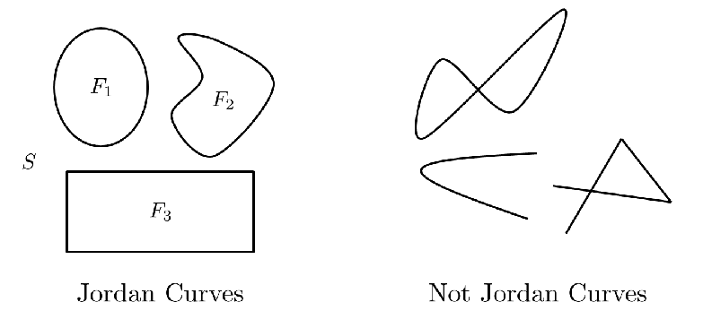
\[\int_{C} f(z) d z\]

Well, the good news is that it is not a mere extension of the real integral. There is more to it ! The first trick is to assume a parameter \(t\) that suitably parametrizes the counterclockwise path around our Jordan curve (google it!) C.

The natural choice is to introduce the parameterization and rewrite the integral as follows :

\[\int_{a}^{b} f(p(t)) p^{\prime}(t) d t\]

Where, \(p(t)\) is a function which returns complex values for real \(t\) which goes from \(a\) to \(b\) along the contour.

Let us introduce the dot product of two complex numbers as the equivalent of the vector dot product i.e. \(u.v = (a + ib).(c + id) = ac + bd\) for complex numbers \(u\) and \(v\). Then, note that the product \(\operatorname{Re}(\bar{u} v)=u \cdot v\) and \(\operatorname{Im}(\bar{u} v)= (iu) \cdot v\).

Now, let us look at the contour integral of the complex conjugate of the function f(p(t)) :

\[I = \int_{a}^{b} \overline{f(p(t))} p^{\prime}(t) d t\]

Using the recently derived relation we can write that the Real and Imaginary parts of the integral are given by :

\[\operatorname{Re}(I)=\int_{a}^{b} f(p(t)) \cdot d p(t) \quad \operatorname{Im}(I)=\int_{a}^{b}(i f(p(t))) \cdot d p(t)\]

A quick observation and you will immediately realize that the Real part is actually the work done over the contour and the Imaginary part is the flux (\(if\) is normal to \(f\)). [ Note: All of this holds if we consider f as a vector field. ]

Source in 2-D Flow

In fluid dynamics, the analysis of 2-D irrotationa and incompressible flows often involves the complex potential \(F = \phi + i\psi\). Where \(\phi\) is the potential function (its gradient gives the velocity field) and \(\psi\) is orthogonal to \(\phi\) and it is known as the stream function (constant \(\psi\) lines are the streamlines).

Using the fact that the velocity field for a source should be proprotional to \(1/r\), it can be shown that the complex potential \(F = k.log(z)\) where \(k\) is a constant.

Furthermore, if one differentiates \(F\) w.r.t \(z\) and gets simplifies the result using the definition of \(\phi\) and \(\psi\), we get that \(\frac{dF}{dz} = F^{\prime} = u - iv\) where \(u\) and \(v\) represent the x and y components of the fluid’s velocity. Therefore, \(\overline{F^{\prime}} = u + iv\) can be seen as the velocity field.

Let us see apply the residue theorem now ! The flux of velocity field integrated over the contour C should give an idea of the strength of the source or in fact, the fluid’s flow rate. The complex conjugate of the velocity field is \(\frac{dF}{dz} = \frac{k}{z}\).

The residue theorem states that the integral of the aforementioned functions is simply equal to \(2\pi.i.k\). Therefore, its imaginary part is \(2\pi.k\). Also, the integral of the velocity field over the contour should be equal to the volume flow rate per unit depth \(= q\) (say).

This example was a simple use-case of a powerful method that can be used to aid the solution of more complicated 2-D fluid flow fields.

Thanks for reading till this point !

Proof of the Residue Theorem : Proof