Problem 11 : Lorenz Equation- Laser problem

Chaos, a weird still fascinating branch of mathematics that deals with nonlinear real systems and gives non-reapeating finite values as solution for a certain set of values of system parameters. To start the disucssion we have to introduce the famous Lorenz equation for atmospheric covection modelling. The most simplified version is

\[\dot{x}=\sigma(y-x) \\ \dot{y}=rx-y-xz \\ \dot{z}=xy-bz \\\]

Where x, y, z are the dynamical variables and \(\sigma\), r, b are the physical parameters. In this post we are going to describe a similar system on the laser physics domain. The problem is taken from the book “Nonlinear Dynamics and Chaos” by Steven Strogatz. So, let’s get started.

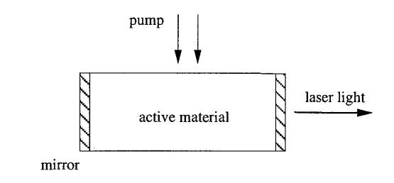
We are going to consider a solid state laser source that started to emit laser light upon excited by an external energy source. The energy will excite the atoms inside the active material and they emit photons of different energies. There exists a threshold limit for the number of excited atoms generated which decide the emitting light will be laser light or not.

This phenomena is governed by the Maxwell-Bloch equation and the simplified version is given below,

\[\dot{E}=\kappa(P-E) \\ \dot{P}=\gamma_1(ED-P) \\ \dot{D}=\gamma_2(\lambda+1-D-\lambda EP) \\\]

Where E,P,D are the dynamical variables and \(\kappa\), \(\gamma_1\), \(\gamma_2\) and \(\lambda\) are the system parameters. The questions are,
(a)Show that the non-lasing state (the fixed point with E* = 0) loses stability above a threshold value of \(\lambda\), which is to be determined. Classify the bifurcation at this laser threshold.
(b)Find a change of variables that transforms the system into a Lorenz system.

Solution

Before proceeding to the solution I will describe the simplified model and solve it. Let’s say the dynamical variable is the number of photons n(t) in the laser field. The expression of n(t) can be written as,

\[\dot{n}=gain-loss \implies \dot{n}=GnN-kn\]

where G is the gain coefficient and k is the loss coefficient. \(N(t)\) is the number of excited atoms in the active material. Physically the gain terms comes from the process of \(\textit{stimulated emission}\) which means the photons coming from the pump excite the atoms to generated more and more photons. Whereas the loss happens when the photons escapes through the endfaces of the laser.

Now both n and N are dependent on time, so, we need to have one more relation. The key physical idea is that the atoms will be down to lower energy state after releasing a photon and then they are unable to emit another photon. This idea suggests that the number of active excited atoms drops as increase in the photon number.

\[N(t)=N_0-\alpha n\]

Where \(N_0\) is the number of excited atoms in absence of laser action(without external pump). Combining the above equations,

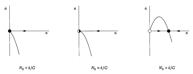
\[\dot{n}=(GN_0-k)n-(\alpha G)n^2\]

Where G>0, k>0 and \(\alpha\)>0.

Considering the phase plot for the dynamical variable n(t) there is a bifurcation at \(N_0=k/G\). Below this \(N_0\) value there will be no laser light emission as all the photons will be out of phase with each other. Beyond this value there is high increase of laser intensity and all the photons will be in the same phase.

Now coming to our actual problem, we have to find the non-lasing state fixed point corresponding to the \(E^*=0\) and then find out the local stability. Now it is evident from the equations that the fixed point will be,

\[E^*=0 \\ P^*=0 \\ D^*=\lambda +1 \\\]

We have to find the Jacobian matrix(Reference) and find the eigen values and corresponding eigen vectors using Wolrfam Alpha computational machine,

\[J=\begin{bmatrix} -1 & 1 & 0 \\ \lambda +1 & -1 & 0 \\ 0 & 0 & -1 \\ \end{bmatrix}\]

Eigen values and Eigen vectors,

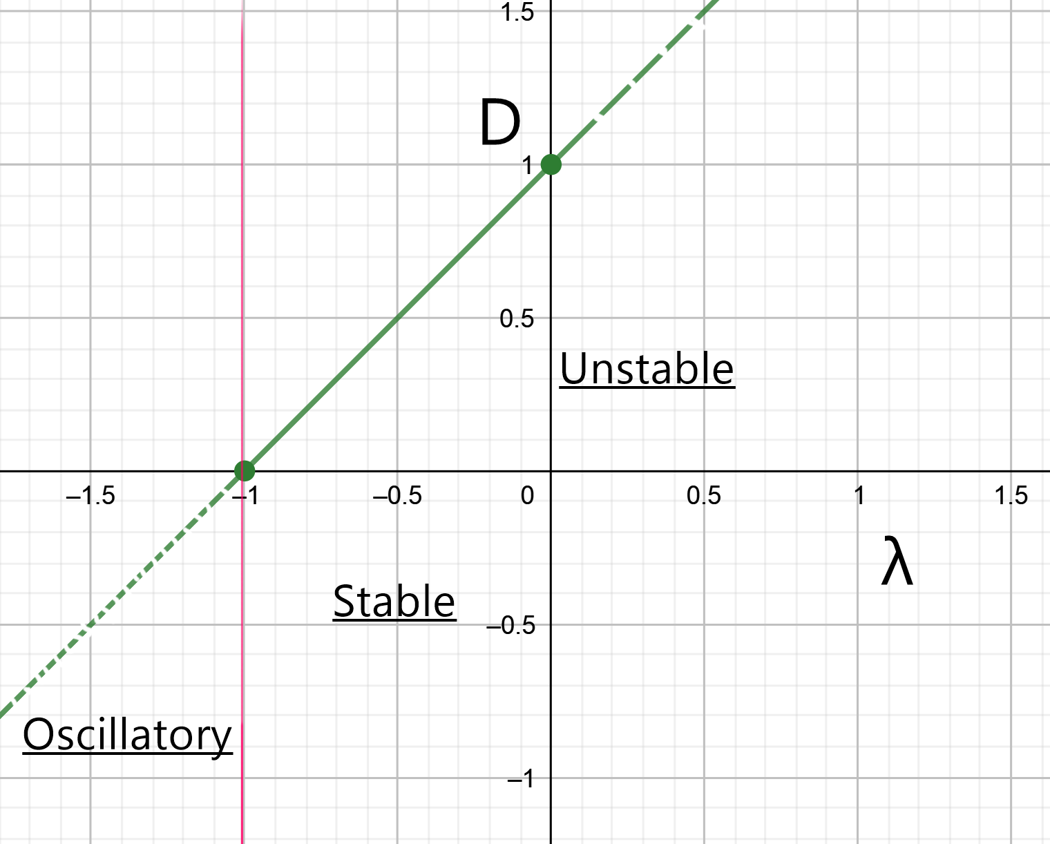
\[\lambda_1= -1, v_1=\begin{pmatrix} 0, & 0, & 1 \end{pmatrix} \\ \lambda_2= -\sqrt(\lambda+1)-1, v_2=\begin{pmatrix} \frac{-1}{\sqrt{\lambda+1}}, & 1, & 0 \end{pmatrix} \\ \lambda_3= \sqrt(\lambda+1)-1, v_3=\begin{pmatrix} \frac{1}{\sqrt{\lambda+1}}, & 1, & 0 \end{pmatrix}\]

We know negative Eigen values denotes the stability of the system and positive Eigen values denotes the unstability of the system along its corresponding Eigen vector. In this case \(\lambda_1\) and \(\lambda_2\) are always negative as the system parameter \(\lambda\) is real and greater than -1. So only \(\lambda_3\) can take the positive value when \(\lambda >0\) and make the system unstable. In other cases the system cease to be stable when \(\lambda\)<-1 because the eigen values become imaginary that changes its behavior to oscillatory.

Surprisingly there are three stability region considering the value of \(\lambda\) and the bifurcaiton diagram shows as follows,

In the second part of our problem the system can be expressed similar to Lorenz’ equation by a simple transformation \(D^\prime=D-(\lambda +1)\). Which give us,

\[\dot{E}=\kappa(P-E) \\ \dot{P}=\gamma_1((\lambda +1)E-P-ED^\prime) \\ \dot{D^\prime}=\gamma_2(\lambda EP-D^\prime) \\\]

Now this system is nonlinear and for certain values of \(\kappa\), \(\gamma_1\), \(\gamma_2\), \(\lambda\) it execute chaotic bevavior that means small change in the initial condition completely change the dynamical evolution of the variables.

The following figure is the solution of Lorenz type equation where the dynamical variables x vs z is plotted. The value of the paramter is taken as, \(\sigma\)=10, r=21 and b=8/3. The blue and red color plots are the two solution of the system with a very minimal difference in the initial condition. You can see after some time both of the solution are showing a completely different nature and at steady state they come to two different fixed points. This shows the fundamental characteristics of Chaos.

If you are interested just like us then trying reading the book ‘Nonlinear Dynamics and Chaos’ mentioned earlier and search for Butterfly Effect.